Defining adjacency
The key in toplogical coloring is the definition of adjacency, to
understand which features are neighboring and could not share the same
color. greedy comes with several methods of defining it. Binary
spatial weights denoting adjacency are then stored as libpysal’s weight
objects.
import geopandas as gpd
import pandas as pd
import numpy as np
from time import time
import seaborn as sns
import matplotlib.pyplot as plt

from shapely.geometry import Point

from greedy import greedy

sns.set()
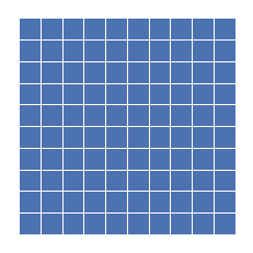
For illustration purposes, let’s generate a 10x10 mesh of squared polygons:
polys = []
for x in range(10):
    for y in range(10):
        polys.append(Point(x, y).buffer(0.5, cap_style=3))
gdf = gpd.GeoDataFrame(geometry=polys)
ax = gdf.plot(edgecolor='w')
ax.set_axis_off()
libpysal adjacency
The most performant way of generating spatial weights is using libpysal contiguity weights. As they are based on the shared nodes or edges, dataset needs to be topologically correct. Neighboring polygons needs to share vertices and edges, otherwise their relationship will not be captured.
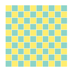
Rook
There are two ways how to define contiguity weights - rook and
queen. Rook identifies two objects as neighboring only if they share
at least on edge - line between two shared points. Use rook if you do
not mind two polygons touching by hteir corners having the same color:
gdf['rook'] = greedy(gdf, sw='rook', min_colors=2)
ax = gdf.plot('rook', edgecolor='w', categorical=True, cmap='Set3')
ax.set_axis_off()
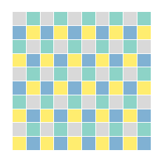
Queen
The default option in greedy is queen adjacency. That identifies
two objects as neighboring if they share at least one point. It ensures
that even poygons sharing only one corner will not share a color:
gdf['queen'] = greedy(gdf, sw='queen', min_colors=2)
ax = gdf.plot('queen', edgecolor='w', categorical=True, cmap='Set3')
ax.set_axis_off()
Intersection-based adjacency
As noted above, if the topology of the dataset is not ideal, libpysal
might not identify two visually neighboring features as neighbors.
greedy can use intersection-based algorithm using GEOS intersection
to define if two features intersects in any way. They do not have to
share any points. Naturally, such an approach is significantly slower
(details below), but it can provide correct adjacency when libpysal
fails.
To make greedy to use this algorithm, one just needs to define
min_distance. If it is set to 0, it behaves similarly to queen
contiguity, just capturing all intersections:
gdf['geos'] = greedy(gdf, min_distance=0, min_colors=2)
ax = gdf.plot('geos', edgecolor='w', categorical=True, cmap='Set3')
ax.set_axis_off()

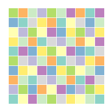
min_distance also sets the minimal distance between colors. To do
that, all features within such a distance are identified as neighbors,
hence no two features wihtin set distance can share the same color:
gdf['dist1'] = greedy(gdf, min_distance=1, min_colors=2)
ax = gdf.plot('dist1', edgecolor='w', categorical=True, cmap='Set3')
ax.set_axis_off()
Reusing spatial weights
Passing libpysal.weights.W object to sw, will skip generating
spatial weights and use the passed object instead. That will improve the
performance if one intends to repeate the coloring multiple times. In
that case, weights should be denoted using GeodataFrame’s index.
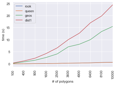
Performance
The difference in performance of libpysal and GEOS-based method is large, so it is recommended to use libpysal if possible. Details of comparison between all methods are below:
times = pd.DataFrame(index=['rook', 'queen', 'geos', 'dist1'])
for number in range(10, 110, 10):
    print(number)
    polys = []
    for x in range(number):
        for y in range(number):
            polys.append(Point(x, y).buffer(0.5, cap_style=3))
    gdf = gpd.GeoDataFrame(geometry=polys)
    timer = []
    for run in range(5):
        s = time()
        colors = greedy(gdf, sw='rook', min_colors=2)
        e = time() - s
        timer.append(e)
    times.loc['rook', number] = np.mean(timer)
    print('rook: ', np.mean(timer), 's; ', np.max(colors) + 1, 'colors')
    timer = []
    for run in range(5):
        s = time()
        colors = greedy(gdf, sw='queen', min_colors=2)
        e = time() - s
        timer.append(e)
    times.loc['queen', number] = np.mean(timer)
    print('queen: ', np.mean(timer), 's; ', np.max(colors) + 1, 'colors')
    timer = []
    for run in range(5):
        s = time()
        colors = greedy(gdf, min_distance=0, min_colors=2)
        e = time() - s
        timer.append(e)
    times.loc['geos', number] = np.mean(timer)
    print('geos: ', np.mean(timer), 's; ', np.max(colors) + 1, 'colors')
    timer = []
    for run in range(5):
        s = time()
        colors = greedy(gdf, min_distance=1, min_colors=2)
        e = time() - s
        timer.append(e)
    times.loc['dist1', number] = np.mean(timer)
    print('dist1: ', np.mean(timer), 's; ', np.max(colors) + 1, 'colors')
10
rook:  0.008332633972167968 s;  2 colors
queen:  0.0067865848541259766 s;  4 colors
geos:  0.18540759086608888 s;  4 colors
dist1:  0.3216702938079834 s;  10 colors
20
rook:  0.023499011993408203 s;  2 colors
queen:  0.02506265640258789 s;  4 colors
geos:  0.7820498943328857 s;  4 colors
dist1:  1.1883579730987548 s;  10 colors
30
rook:  0.09070181846618652 s;  2 colors
queen:  0.05646052360534668 s;  4 colors
geos:  1.4737992763519288 s;  4 colors
dist1:  2.313761281967163 s;  10 colors
40
rook:  0.1293130874633789 s;  2 colors
queen:  0.08214569091796875 s;  4 colors
geos:  2.6077350616455077 s;  4 colors
dist1:  4.236755275726319 s;  10 colors
50
rook:  0.1469170093536377 s;  2 colors
queen:  0.16109180450439453 s;  4 colors
geos:  4.08953275680542 s;  4 colors
dist1:  6.589194393157959 s;  10 colors
60
rook:  0.25732903480529784 s;  2 colors
queen:  0.25914812088012695 s;  4 colors
geos:  7.026346206665039 s;  4 colors
dist1:  10.011457777023315 s;  10 colors
70
rook:  0.29179821014404295 s;  2 colors
queen:  0.3061429500579834 s;  4 colors
geos:  8.105659198760986 s;  4 colors
dist1:  12.690713024139404 s;  10 colors
80
rook:  0.40609278678894045 s;  2 colors
queen:  0.37023115158081055 s;  4 colors
geos:  10.018446493148804 s;  4 colors
dist1:  16.996356391906737 s;  10 colors
90
rook:  0.5523331642150879 s;  2 colors
queen:  0.5231795310974121 s;  4 colors
geos:  13.362245750427245 s;  4 colors
dist1:  19.79914846420288 s;  10 colors
100
rook:  0.632891035079956 s;  2 colors
queen:  0.6089587688446045 s;  4 colors
geos:  15.45732364654541 s;  4 colors
dist1:  24.436386251449584 s;  10 colors
Comparison of time needed to generate greedy coloring using each of the methods above shows the big difference between GEOS and libpysal:
ax = times.T.plot()
ax.set_ylabel('time (s)')
ax.set_xlabel('# of polygons')
locs, labels = plt.xticks()
plt.xticks(locs, (times.columns ** 2), rotation='vertical')
Plotting without the GEOS methods, the difference between queen and
rook is minimal:
ax = times.loc[['rook', 'queen']].T.plot()
ax.set_ylabel('time (s)')
ax.set_xlabel('# of polygons')
locs, labels = plt.xticks()
plt.xticks(locs, (times.columns ** 2), rotation='vertical')
